Show LLR-TimeMachine Interface Example

About LLR-TimeMachine

LLR-TimeMachine is a spectral chronology visualization tool for LLR outputs.

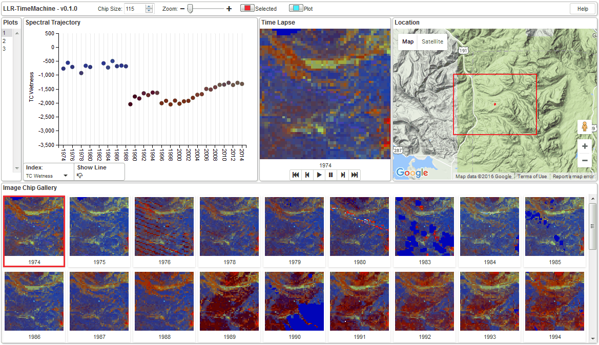
It allows you to view the spectral history of selected pixels as a time series plot and a series of image subsets for the 127 x 127 pixel area surrounding each selected pixel. It provides a time lapse video of the image subset series and a Google Earth representation of the area surrounding the plot. It is web-based, using JavaScript, HTML, and CSS. It relies on several JavaScript packages that are accessed from online sources, therefore, you must be connected to the internet to use the application.

The application is interactive. You can zoom the image subsets, change spectral indices, zoom the time series plot Y axis, change the size of the image subsets, and add time series segments to help interpret the spectral history.

---

LLR-TimeMachine demonstration

Click this link to load a demo version of the application. When the page loads, click the plot ID numbers in the Plots section of the interface (upper-left) to load example data.

---

Download LLR-TimeMachine

Click on a version link and download the HTML file to your computer. Copy/paste or move the downloaded file to any LLR-TimeMachine data directory and open it from that location to load the application - it hitches up to data in that folder. More details on how to setup and run LLR-TimeMachine are included in the walkthrough below. Check back periodically to see if there are updates and bug fixes. If there is an update from the version you have, simply download the new version and replace your old version with the new one in your LLR-TimeMachine data directories.

It has been tested using Firefox, Google Chrome, Opera, and Internet Explorer. Application appearance varies slightly among the browsers. We recommend Firefox, Google Chrome, or Opera. It was designed and tested most comprehensively using Firefox. We have noticed a small problem with the spectral segmentation line when using Google Chrome, we are working on it - not a serious problem, it still works in Chrome.

---

Instructions for setting up LLR-TimeMachine

Outline

1. Complete all of the steps to produce LandsatLinkr annual composites
2. Make a comma delimited file including plot number and x-y coordinates of the pixels you want to view with LLR-TimeMachine
3. Run the llr_time_machine R script to creates the LLR-TimeMachine data.
4. Move or copy/paste the LLR-TimeMachine HTML file into the LLR-TimeMachine data folder
5. Open the LLR-TimeMachine HTML file
6. Use the "Help" button in the LLR-TimeMachine application to find out about the functionality

Walkthrough

1. Use the Guide to get through running all the LandsatLinkr steps. You need to complete image preparation through compositing

2. You need to make a comma delimited file that contains the plot number and x-y coordinates for a series of pixels you want to view in LLR-TimeMachine. They are used to extract the data from the LLR annual composite images and populate some fields in the application

Create the plots file in a text editor like Notepad++ or in Microsoft Excel. In a text editor the format would be:

plotID,x,y
1,-1177707,2527795
2,-1176447,2536015
3,-1168707,2529235				

...and in Excel:

plotID	x	y
1	-1176447	2536015
2	-1177707	2527795
3	-1168707	2529235

Enter as many coordinates as you like. Keep in mind that the coordinates must be in the same projection as the image data and that the points fall within the bounds of the composite imagery you are creating LLR-TimeMachine data for. Coordinates can be retrieved from any GIS that the composite image data is loaded into. Save the file to your computer as a .csv file. You might create a directory on your system called "llr_timemachine" and write the file to this location with a name that is unique to a project you are working on. Something like:

"C:/mock/llr_timemachine/project_1/project_1_plots.csv"

The full directory path to this file will be given as an input to an R function called in the next step, so keep its location in mind.

3. Create LLR-TimeMachine application data for the points you provided in the plots file in step 2. To do this you will call the llr_time_machine function from the LandsatLinkr package in R. This function is only included in LandsatLinkr version >= 0.3.0, so download new code if you have an older version. Here is the function call and the parameter definitions:

llr_time_machine(imgdir, outdir, coordfile)

where,

imgdir equals a character string for the full directory path to you LLR composites output folder that correspond to the coordinates you entered in the plots file in step 2. This directory was specified when you ran the "Compositing" step of LLR. It is important that this directory contain folders titled: "tca", "tcb", "tcg", "tcw", which indicates composite imagery was created for all tasselled cap spectral indices. The program will not run if these outputs do not exist - the LLR-TimeMachine application requires them.

outdir equals a character string for the full directory path to the location you want your LLR-TimeMachine data written to. For the above example project plots file specified in step 2, I would set it as:

"C:/mock/llr_timemachine/project_1"

coordfile equals a character string for the full file path to the plots file you created in step 2. As in:

"C:/mock/llr_timemachine/project_1/project_1_plots.csv"

Putting it all together, the full call, including loading the LandsatLinkr library would look something like:

library(LandsatLinkr)
llr_time_machine(imgdir="C:/mock/llr_composites/project_1", outdir="C:/mock/llr_timemachine/project_1", coordfile="C:/mock/llr_timemachine/project_1/project_1_plots.csv")

After the function completes its process it will have placed a JavaScript file in the outputs directory titled LLRtimeMachine.js and created a sub-directory called imgs, where it has created a series of PNG image files, one for each plot in the plots list. The directory structure looks like this:

 project_1
    imgs
       plot_1_chipstrip.png
       plot_2_chipstrip.png
       plot_3_chipstrip.png
       ...
    LLR-TimeMachine.js

4. Get the LLR-TimeMachine HTML file into the data folder. This file is the file you downloaded from the Download section above. Get this file into LLR-TimeMachine output folder at the same level as the LLRtimeMachine.js file just previously described. The LLR-TimeMachine HTML file will hitch up to the LLRtimeMachine.js file and the PNG files in the imgs directory. Your LLR-TimeMachine directory structure should now look like this:

 project_1
    imgs
       plot_1_chipstrip.png
       plot_2_chipstrip.png
       plot_3_chipstrip.png
       ...
    LLR-TimeMachine.js
    LLR-TimeMachine-v0.1.0.html

5. Open the LLR-TimeMachine HTML file. Navigate to the LLR-TimeMachine data directory and open the HTML file. It will open even if you are not connected to the internet, but the application will not work properly because it relies on some scripts that are hosted on the net, so make sure you are connected. The HTML file will retrieve data from the LLR-TimeMachine.js file and the imgs directory to populate the application.

6. Once the application has loaded you can find out about its functionality from the Help button on the upper-right part of the interface. A series of plots should have loaded into the Plots section of the interface. Click on these to load the data for each coordinate you provided.