Introduction
About LandsatLinkr
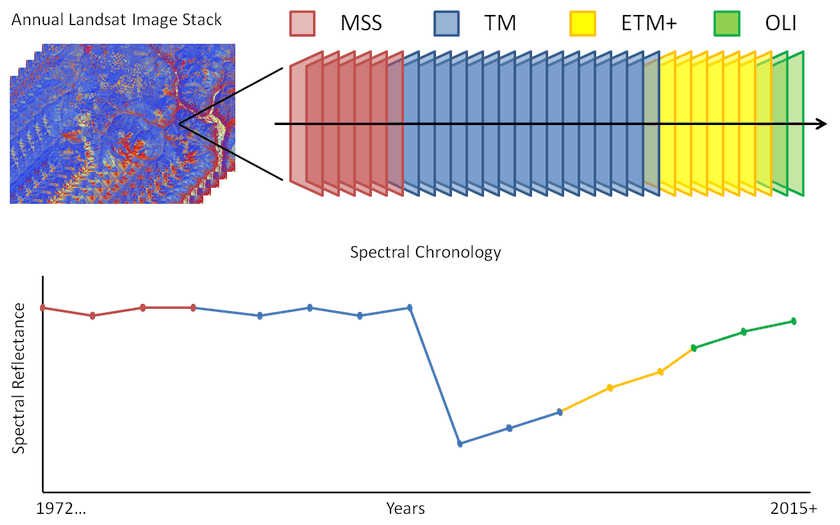
LandsatLinkr (LLR) is an automated Landsat image processing system designed to spatially and spectrally link MSS, TM, ETM+, and OLI images through time. It efficiently processes hundreds of images to produce annual cloud-free image composites from which to build 42+ year spectral chronologies (Figure 1). The resulting spectrally consistent composite images can be used individually as inputs to mapping or modeling projects, to investigate simple image-to-image change, or as inputs to complex change detection algorithms such as LandTrendr.
LLR takes hundreds of images and automatically completes the following steps:
- Decompresses
- Reprojects
- Stacks image bands
- Creates cloud masks
- Improves MSS georegistration accuracy
- Applies atmospheric correction
- Resamples MSS images to 30m
- Spectrally calibrates MSS data to TM data
- Spectrally calibrates OLI data to ETM+ data
- Creates annual cloud-free image composites and stacks
Each step produces outputs which are independently useful (following list), so even if you only need a couple of images processed to surface reflectance and do not care about annual composites or time series stacks, LLR is still relevant, though the true benefit is in large volume processing.
MSS data outputs
- 4-band DN raster stacks
- 4-band radiance raster stacks
- 4-band atmospherically corrected surface reflectance raster stacks
- 3-band calibrated tasseled cap raster stacks
- 1-band calibrated tasseled cap angle rasters
- 1-band cloud and shadow mask rasters
TM/ETM+ data outputs
- 6-band atmospherically corrected surface reflectance (LEDAPS) raster stacks
- 3-band tasseled cap raster stacks
- 1-band cloud and shadow mask rasters
OLI image data outputs
- 7-band atmospherically corrected surface reflectance (L8SR) raster stacks
- 3-band ETM+ -calibrated tasseled cap raster stacks
- 1-band ETM+ -calibrated tasseled cap angle rasters
- 1-band cloud and shadow mask rasters
Composite data outputs
- 1-band annual tasseled cap brightness rasters
- 1-band annual tasseled cap greenness rasters
- 1-band annual tasseled cap wetness rasters
- 1-band annual tasseled cap angle rasters
- Multi-band tasseled cap brightness time series raster stack
- Multi-band tasseled cap greenness time series raster stack
- Multi-band tasseled cap wetness time series raster stack
- Multi-band tasseled cap angle time series raster stack
LandsatLinkr is written in the R programming language and distributed as an R package. The system features an interactive interface for simple operation with no R experience needed. It provides an option to run the system in parallel using 2 cores to reduce standard processing time by half.
It was developed for landscape change research as a way to easily incorporate the entire Landsat archive into spatially and spectrally consistent 42+ year time series stacks. As such, it is constantly changing to meet new needs and is not considered end-point software. However, the outputs are generically useful for nearly all applications of Landsat time series data, so we provide it freely, encourage its use, and welcome any feedback regarding bugs and suggested improvements - see Contact page for email address.
LandsatLinkr workflow
MSS, TM, ETM+, and OLI sensors produce somewhat different data. Though part of the same Landsat family, with similar mission objectives, technology enhancements over time have led to a divergence in image attributes between sensors (Table 1). LLR bridges the difference between sensors by spatially and spectrally aligning the data through georegistration improvement, resampling, and spectral index modeling and calibration. The processing procedures are based on established methods and executed with a high degree of automation and standardization. A brief description of the LLR workflow follows. Step-by-step instructions for setup and executing are presented in the Setup and Running LandsatLinkr sections.
| Attribute | MSS | TM | ETM+ | OLI |
|---|---|---|---|---|
| Ultra-blue band (micrometers) | - | - | - | 0.43-0.45 |
| Blue band (micrometers) | - | 0.45-0.52 | 0.45-0.52 | 0.45-0.51 |
| Green band (micrometers) | 0.50-0.60 | 0.52-0.60 | 0.52-0.60 | 0.53-0.59 |
| Red band (micrometers) | 0.60-0.70 | 0.63-0.69 | 0.63-0.69 | 0.64-0.67 |
| NIR band (micrometers) | 0.70-0.80 | 0.76-0.90 | 0.77-0.90 | 0.85-0.88 |
| NIR band (continued) (micrometers) | 0.80-1.10 | |||
| SWIR 1 band (micrometers) | - | 1.55-1.75 | 1.55-1.75 | 1.57-1.65 |
| SWIR 2 band (micrometers) | - | 2.08-2.35 | 2.09-2.35 | 2.11-2.29 |
| Cirrus band (micrometers) | - | - | - | 1.36-1.38 |
| Radiometric Resolution (bit) | 8* | 8 | 8 | 12 |
| Spatial resolution (m) | 60** | 30 | 30 | 30 |
| Temporal resolution (days) | 18 & 16 | 16 | 16 | 16 |
| Years of operation | 1972-1992 | 1982-2012 | 1999-... | 2013-... |
LandsatLinkr has six major processing steps (Figure 2):
- Preparing MSS imagery
- Preparing TM/ETM+ imagery
- Preparing OLI imagery
- Calibrating MSS to TM imagery
- Calibrating OLI to ETM+ imagery
- Annual cloud-free image compositing
The external inputs include:
- A temporal series of LPGS MSS images for a given Landsat scene
- An MSS scene-corresponding digital elevation model (DEM)
- A temporal series of LEDAPS TM/ETM+ images for a given Landsat scene
- A temporal series of L8SR OLI images for a given Landsat scene
The remaining inputs in steps 4-6 are created internally and accessed automatically
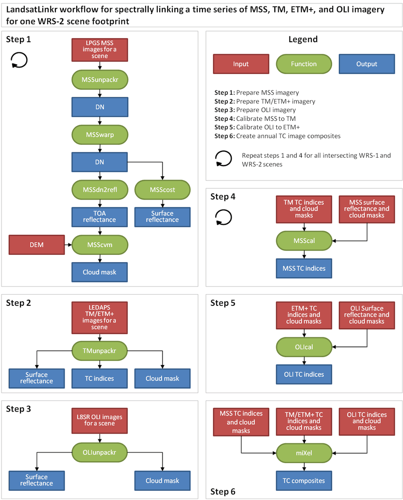
Step 1 - prepare MSS imagery
Every LPGS MSS image for a particular Landsat scene (WRS Landsat path/row footprint) is decompressed, stacked, and reprojected, renamed, and organized into a defined directory structure (MSSunpackr). Georegistration accuracy is assessed from image metadata and enhanced using an image-to-image tie point search and warp procedure (MSSwarp) if scene-level RMSE <= 0.75. All images are then converted to units of top-of-atmosphere (TOA) reflectance (MSSdn2rad) and surface reflectance (MSScost). The radiance images along with a scene-corresponding DEM are then used in a cloud masking procedure (MSScvm) to create raster images that identify clear-view and obscured pixels for later use in cloud-free compositing. Finally, the TOA reflectance images and the cloud masks are resampled to 30m to match the spatial resolution of the TM, ETM+, and OLI data.
Step 2 - prepare TM/ETM+ imagery
Every LEDAPS TM/ETM+ image for an intersecting MSS scene processed in Step 1 will be decompressed, stacked, and reprojected. From the surface reflectance image stack, a 3-band Tasseled Cap transformation raster stack is created. Finally, the included Fmask cloud mask is aggregated to identify clear-view and obscured pixels with the same designation as the MSS masks created in Step 1. All image data are renamed and organized into a defined directory structure. The TMunpackr function is responsible for procedures in Step 2.
Step 3 - prepare OLI imagery
Every L8SR OLI image for an intersecting TM/ETM+ scene processed in Step 2 will be decompressed, stacked, and reprojected. The included Fmask cloud mask is aggregated to identify clear-view and obscured pixels with the same designation as the MSS masks created in Step 1. All image data are renamed and organized into a defined directory structure. The OLIunpackr function is responsible for procedures in Step 3.
Step 4 - calibrate MSS to TM
The MSScal function develops models to predict TM spectral indices from MSS surface reflectance bands based on the relationship between coincident MSS and TM dates for years 1982-1992. Specifically, models are created for Tasseled Cap Brightness, Greenness, Wetness, and Angle. The models are then applied to all MSS images in the model reference scene.
Note: steps 1 and 3 are repeated as necessary for all intersecting scenes in a project study area. This is particularly relevant for including the multiple Landsat 1-3 WRS-1 scenes that intersect Landsat 4-8 WRS-2 scenes. See section Setup processing directories for more details on the World Reference System version difference and how they affect the LLR process.
Step 5 - calibrate OLI to ETM+
The OLIcal function (very similar to the MSScal in Step 4) develops models to predict ETM+ spectral indices from OLI surface reflectance bands based on the relationship between near-date OLI and ETM+ images for the period 2013-present. Specifically, models are created for Tasseled Cap Brightness, Greenness, Wetness, and Angle. The models are then applied to all OLI images in the model reference scene.
Step 6 - create annual image composites
Step 6 produces annual cloud-free image composites for all spatially intersecting images in a given region of interest. The miXel function searches provided directories for images to composite and sorts them into groups by year. For all images in each year group, cloud masks are applied to set obscured pixels to the background (NA) value and then the year composite is calculated from the per-cell mean value of overlapping images.
Each LLR processing steps is run with a single R function called run_landsatlinkr().
Each step of the process is run independently and must be completed in order.
System requirements
Computer
LandsatLinkr was developed and tested on computers running Windows 7 64-bit OS with >= 8 GB of RAM.
Data storage
2 TB of data storage is recommended for processing a single WRS-2 scene project with ~250 images.
Software
- R
- RStudio
- GDAL
Setup
Install software
LLR requires R, RStudio, and GDAL programs be installed on your computer. R is a free computer programming language for statistical computing and graphics. RStudio provides a convenient frontend interface to the R environment. GDAL is a program for reading, writing, and manipulating geospatial data.
If you don't already have a current version of these programs you'll need to download and install them to your computer.
R
Follow the install directions on the R website
RStudio
Follow the install directions on the RStudio website
GDAL
There are numerous ways you can install GDAL, the following is one example.
- Go to http://www.gisinternals.com/release.php
- Click on the Downloads link for the version that best matches your system (we use MSVC 2010 - x64)
- Download the Generic installer for the GDAL core components
- Run the installer
- Include GDAL in your system's environmental variable PATH
- Open Windows Control Panel and select System
- Click on Advanced system settings
- Click the Environmental Variables... button
- Under System variables, scroll down to the Path variable and click on it to highlight it
- Click the edit button
- Get your cursor to the end of the line, add a semi-colon (;) and add the path to the GDAL installation location. Example: C:\GDAL (this may not actually be the location on your system)
Install LandsatLinkr
LandsatLinkr is written in the R programming language and its commands are entered and run through RStudio. R has many user-developed packages to handle most data concerns. LandsatLinkr is one such package and it relies on several other useful packages that are automatically downloaded and installed upon running LandsatLinkr. Once R and RStudio are set up you'll need to install the LandsatLinkr package.
1. Open the RStudio program and find the console command prompt.
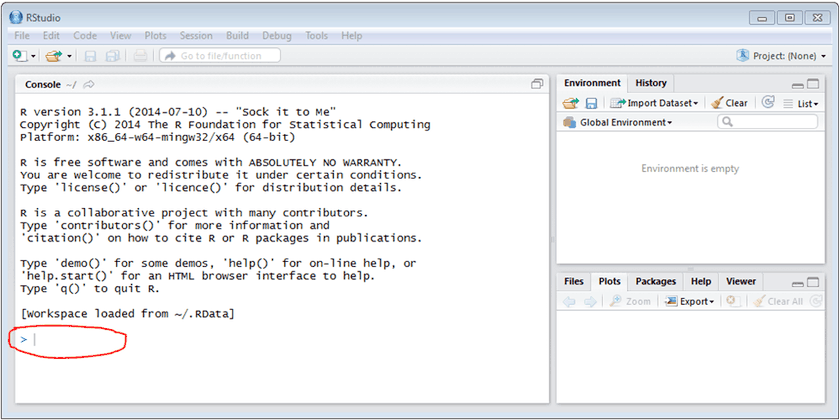
The red circle in Figure 3 is where you will be entering function calls and their arguments - example:
this_function(argument1 = input, argument2 = NULL)
Upon pressing enter the function will execute - not in this case - this is a mock example.
2. Install the LandsatLinkr package. To install the package from the GitHub repository, copy and paste the following code lines into the RStudio command prompt and press enter. Alternatively, use the lines provided on the LLR download page. Check occasionally for version updates, which include bug fixes and enhancements.
download.file("https://github.com/jdbcode/LandsatLinkr/releases/download/0.5.0-beta/LandsatLinkr_0.5.0.zip", "LandsatLinkr")
install.packages("LandsatLinkr", repos=NULL, type="binary")
install.packages(c("raster","SDMTools","doParallel","foreach","plyr","gdalUtils","rgdal","igraph","MASS"))
3. Once the package has been installed it must be loaded into the current R session. Loading the package allows R to access the installed code. This procedure must be done each time a new session is started. The first time that the LLR package is loaded it will automatically prompt R to download and install several dependent packages. To load the LLR package, type or copy the following line into the command prompt and press enter.
library(LandsatLinkr)
LandsatLinkr is now ready to run on your machine.
Setup processing directories
Keeping data organized with standard directory structures and file naming conventions is important to automation and data management. Before beginning a project you must create four directories for:
- MSS WRS-1 images
- MSS WRS-2 images
- TM/ETM+ WRS-2 images
- OLI WRS-2 images
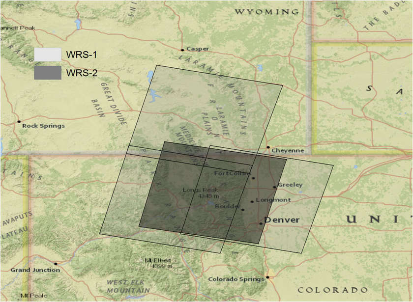
The image sensor (MSS, TM/ETM+, and OLI) is an obvious distinction for keeping Landsat data organized (we group TM and ETM+ together because they have nearly identical properties), but WRS-1 and WRS-2 scene grid designations are equally as important. WRS refers to the World Reference System. It is a standard path/row grid that defines the spatial extent of each Landsat scene footprint on Earth's surface. Unfortunately, the two grid systems do not have the same path/row alignment or numbering scheme because of differences in satellite obits. This means that including the full temporal archive for a single WRS-2 scene requires that multiple WRS-1 scenes are processed and included in calibration and compositing. Landsat 1-3 (MSS only) use WRS-1 and Landsat 4-8 (MSS 4-5, TM, ETM+, and OLI) use WRS-2. Figure 4 shows an example of the mismatch in the alignment and path/row numbering for a single WRS-2 scene of interest. For more information on the World Reference Systems please visit this site.
Determining which scenes are needed to process a region of interest for the full 42+ year history is the first step in setting up a processing directory structure. This can be accomplished several ways. USGS provides ArcGIS shapefiles for both WRS-1 and WRS-2 grids that can be used to identify which scenes are needed to cover your region of interest. The files can be downloaded here. Alternatively, the Earth Science Data Viewer provided by the Global Land Cover Facility can also be used to figure this out using the following steps:
- Go to the Earth Science Data Viewer page and use Map Search to zoom into your region of interest
- Click on the Map Layers tab at the top of the viewer and highlight WRS-2 and click Update Map
- Determine which WRS-2 path/row covers your region of interest
- Click on the Path/Row tab at the top of the viewer and type in the path and row for the WRS-2 scene of interest (start and end as the same) and click Update Map
- Go back to the Map Layers tab and highlight WRS-1 and click Update Map and then note which WRS-1 scenes intersect the outlined WRS-2 scene.
Once you know what scenes you'll need, you can create the LandsatLinkr base directory structure (Figure 5).
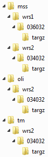
Each scene should have the following directory path that first defines what sensor it comes from, then which WRS system (1 or 2) the data is from, followed by the 6 digit path/row label, and finally a folder to place the downloaded images in (targz):
<drive><...><sensor><wrs><ppprrr><targz>
Where:
drive = the drive letter for the disk you are writing to
... = any other designation you want (optional)
sensor = what sensor collected the data (mss, tm, or oli - tm is used for both TM and ETM+)
wrs = what WRS grid system delineates the scene ("wrs1" or "wrs2")
ppprrr = what is the 6-digit scene path/row code (example: "036034")
targz = a folder called targz where the downloaded images are to be placed
Example: L:/landsat/mss/wrs1/036032/targz
There are four main directories defined by all combinations of sensor and WRS grid type:
*/mss/wrs1
*/mss/wrs2
*/tm/wrs2
*/oli/wrs2
Within each of these main directories you may have several scene directories, each with their own targz folder.
For all the scenes identified intersecting your region of interest, create directories for them following the LLR directory structure.
Download Landsat images
All images are downloaded from the USGS Earth Explorer website. MSS images should be of the Pre-Collection 1 LPGS product type and surface reflectance for TM/ETM+ and OLI of the Collection 1 Higher-Level product type. For Landsat MSS 1-3 (WRS-1), MSS 4-5 (WRS-2), TM, ETM+, and OLI you will select images to include in separate processing orders. You will need an Earth Explorer user account to download images. You can register for one on the home page, if you don't already have an account.
Currently, LLR is designed to work with summer images (June-Aug. northern hemisphere and Dec.-Feb. in southern hemisphere). Using this short time window during the summer reduces the ephemeral spectral inter- and intra-annual variability due to phenology, snow cover, and sun angle. We are working on ways to allow more flexibly in date range, but for now it is advisable to use only data from summer months. Use good judgement for high and low latitude scenes.
MSS images
- At the Earth Explorer homepage, within the Search Criteria tab and under the Data Range tab select only summer months from the Search months drop down menu.
- Under the Results Options tab increase the Number of records to return to 1,000 (ensures that the image list is not truncated) and then press the Data Sets button
- Expand the Landsat Archive menu, then the Pre-Collection Level-1 menu and check the L1-5 MSS box and click the Additional Criteria tab.
- Scroll down to the WRS Type menu and select the WRS type that corresponds to the scene you intend to download. WRS for Landsat 1, 2, & 3 (WRS-1) or WRS for Landsat 4 & 5 (WRS-2).
- Under the WRS Path and WRS Row fields enter the associated path and row number for the scene of interest.
- Scroll down to the Data Type Level 1 menu and select MSS L1T and then click the Results button
- For each image in the list that is not completely clouded select either the Add to Bulk Download button or Add to Cart button and then press the View Item Basket
- Review your selected images to ensure that you have images for only the intended scene for summer months for years 1972-1982 (WRS-1) or 1982-1992 (WRS-2) (may be some missing years for lack of data) and then press the Proceed to Checkout button.
- Press the Submit Order button.
- You will receive an order confirmation email. If the order includes images added as Bulk Download they are immediately available. Follow the instructions in the email to download them. If there are images that were added to the cart for processing, then you will be instructed to wait for a second email indicating that processing is complete.
Repeat these steps for all MSS scenes (WRS-1 and WRS-2), adjusting the WRS type and path/row entries as needed in steps 4 and 5.
Once images have been downloaded move them to the targz folder for the appropriate sensor, WRS type, and path/row identification.
Downloading TM/ETM+
Downloading TM/ETM+ images requires the same steps as downloading MSS images, but with a different data set selection.
- At the Earth Explorer homepage, within the Search Criteria tab and under the Data Range tab select only summer months from the Search months drop down menu.
- Under the Results Options tab increase the Number of records to return to 1,000 (ensures that the image list is not truncated) and then press the Data Sets button
- Expand the Landsat menu, then the Landsat Collection 1 Level-2 menu and check the Landsat 4-5 TM C1 Level-2 box and click the Additional Criteria tab.
- Under the WRS Path and WRS Row fields enter the associated path and row number for the scene of interest.
- Scroll down to the Collection Category menu and select Tier 1 and then click the Results button
- For each image in the list that is not completely clouded select either the Add to Bulk Download button or Add to Cart button and then press the View Item Basket
- Review your selected images to ensure that you have images for only the intended scene for summer months for years 1982-2011 (TM) or 1999-present (ETM+) (may be some missing years for lack of data) and then press the Proceed to Checkout button.
- Press the Submit Order button.
- You will receive an order confirmation email. If the order includes images added as Bulk Download they are immediately available. Follow the instructions in the email to download them. If there are images that were added to the cart for processing, then you will be instructed to wait for a second email indicating that processing is complete. When processing is complete follow instructions for downloading. If the email does not indicate the option to bulk download the files you can use a third party downloading utility such as DownThemAll for the Mozilla Firefox browser to efficiently retrieve all hyperlinked files on the image download list page.
Repeat these steps to place an order for ETM+ images with exceptions for step 3 where you will select the Landsat 7 ETM+ C1 Level-2 option instead of Landsat 4-5 TM C1 Level-2. Always make sure to select Tier 1 as the Collection Category (it has been terrain corrected - LLR will not process Tier 2).
Once images have been downloaded move them to the targz folder for the appropriate sensor, WRS type, and path/row identification.
Downloading OLI
Downloading OLI images requires the same steps as downloading TM/ETM+ images, but with a different data set selection.
Exceptions to the TM/ETM+ download instructions are needed for steps 3 where you will select the Landsat 8 OLI/TIRS C1 Level-2 option instead of TM or ETM+. When choosing options under the Additional Criteria tab, make sure that you only select OLI under the Sensor Identifier list. Also make sure to select Tier 1 under the Collection Category section (it has been terrain corrected - LLR will not process L1G).
Image information
Please see the hyperlinked USGS product guides for more information regarding image processing of LPGS MSS and CDR Surface Reflectance TM/ETM+ and OLI data.
Downloaded images are named with a unique identity that contains basic information on each image. All components of the image ID, except for ground station and version, are maintained throughout the production of derived data in the LLR process (more on this in Outputs section).
Landsat Image Identifier: LXSPPPRRRYYYYDDDGSIVV
Where:
- L = Landsat
- X = Sensor (M = MSS(1-3 WRS-1) & (4-5 WRS-1), T = TM(4-5 WRS-2), E = ETM(7 WRS-2), O = OLI(8 WRS-2))
- S = Satellite
- PPP = WRS Path
- RRR = WRS Row
- YYYY = Year of Acquisition
- DDD = Day of Acquisition Year
- GSI = Ground Station Identifier
- VV = Version
Digital elevation model
A digital elevation model (DEM) is needed for processing both MSS WRS-1 and MSS WRS-2 scenes. It is used during the cloud masking procedure to correct for topographic illumination and identifying water. The extent of the DEM should be larger than its corresponding scene (the LLR program will crop it on-the-fly as needed). So depending on what DEM product you use, you may need to mosaic several together. The DEM should be between 30 and 90 meter resolution. When preparing MSS images, LLR will ask you for its directory location and then it will automatically resample, reproject, and crop it to match a given scene. A good source for DEMs is the Global Landcover Facility site, which distributes SRTM data as Landsat WRS-2 footprints. Use the Filled Finished-B product at 1 arc second (30 meter) where possible and the Filled Finished-B product at 3 arc seconds (90 meter) elsewhere. You can use other data sources, but SRTM has the advantage of being a global product with standard processing and void filling. The program-prepared DEM files (reprojected and resampled to match for MSS data) will be written to a new directory called topo inside of the relevant MSS scene folder.
A helper function is provided to make creating DEM mosaics really easy. See the mosaic_dems function in
the LandsatLinkr helper functions section.
We recommend that you create one DEM per WRS scene that is included in your project. This includes all WRS-1 and WRS-2 scenes in your region of interest.
Selecting a geographic projection
Projections transform the curved, 3-dimensional shape of the Earth to a flat 2-dimensional surface, which simplifies its representation for display and computation. Landsat USGS Earth Explorer images are delivered in the Universal Transverse Mercator (UTM) projection (Polar Stereographic projection for scenes with a center latitude greater than or equal to -63.0 degrees) using the World Geodetic System (WGS) 84 datum. This projection is fairly specific to small geographic regions, with different parameters for each UTM zone. This is not ideal for LLR projects, since there is high potential for including multiple scenes that may have different projections, which makes spectral harmonization and mosaicking difficult.
In LLR we have you define the projection that will be applied to all images in the project. Do some research to figure out what projection is best for your region - what projection are other data you might be using in? It's important that whatever projection you use preserves area. If you use the image data to classify land cover and then summarize the area of each class in the image, you want to ensure that area is equivalent over the entire image. We recommend the Albers Equal Area Conic projection. The parameters can be adjusted to suit local to continental regions.
When you run the LLR unpacking steps you will be prompted to define a projection to use by declaring a PROJ.4 string. You can find an extensive list of projections at www.spatialreference.org. Use the search option to find named projections and regions, or scroll through the lists until you find what you are looking for. Click on the projection link and then click on the Proj4 link. Copy and paste the projection string into a text file and save it for reference and easy access when you begin running LLR.
Here are a few PROJ.4 examples:
North American Albers Equal Area Conic:
+proj=aea +lat_1=29.5 +lat_2=45.5 +lat_0=23 +lon_0=-96 +x_0=0 +y_0=0 +ellps=GRS80 +datum=NAD83 +units=m +no_defs
Africa Albers Equal Area Conic:
+proj=aea +lat_1=20 +lat_2=-23 +lat_0=0 +lon_0=25 +x_0=0 +y_0=0 +ellps=WGS84 +datum=WGS84 +units=m +no_defs
Europe Albers Equal area Conic:
+proj=aea +lat_1=43 +lat_2=62 +lat_0=30 +lon_0=10 +x_0=0 +y_0=0 +ellps=intl +units=m +no_defs
China Albers Equal Area Conic:
+proj=aea +lat_1=27 +lat_2=45 +lat_0=35 +lon_0=105 +x_0=0 +y_0=0 +ellps=WGS84 +datum=WGS84 +units=m +no_defs
South America Albers Equal Area Conic:
+proj=aea +lat_1=-5 +lat_2=-42 +lat_0=-32 +lon_0=-60 +x_0=0 +y_0=0 +ellps=aust_SA +units=m +no_defs
Canada Albers Equal Area Conic:
+proj=aea +lat_1=50 +lat_2=70 +lat_0=40 +lon_0=-96 +x_0=0 +y_0=0 +ellps=GRS80 +datum=NAD83 +units=m +no_defs
NAD83 UTM zone 10N:
+proj=utm +zone=10 +ellps=GRS80 +datum=NAD83 +units=m +no_defs
***It is important to use the exact same PROJ.4 projection definition within a project any time you are requested to define it by LLR.
Running LandsatLinkr
Before running LLR make sure you've done the following:
- Downloaded and installed all required software
- Created LLR directory structures
- Downloaded the correct image types from Earth Explorer
- Filled the targz folders within the LLR directory with *.tar.gz images recieved from USGS
- Created a separate DEM that is greater in extent then each of your MSS path/row scenes
- Selected a geographic projection and determined its PROJ.4 string definition
LLR is run with a single R function run_landsatlinkr. It activates an interactive interface where questions and lists of
options will be displayed in the RStudio console. You'll simply type a number to select an option, type and enter brief text, and use Windows
directory pop-ups to select files and folders. Note that after each selection, the LLR interface will verify your selection. Here is an
example of a verification:
Selection: 1
[1] "You have selected: Prepare MSS"
Is that correct?

1: Yes
2: No
3: Exit
If the selection matches your intention, press 1 for Yes, 2 for No, or 3 for Exist.
If you select No, the program will allow you to redefine the selection, if Yes, the program will continue, and if
No, the program will end.
These verifications can be a bit annoying, but it is better than the alternative of accidentally making the wrong selection and having to completely restart the process, or not realize you've made the wrong selection until much processing time as passed.
***Before running any functions, ensure that LLR is loaded in your current R session. Type the following command into the console and press enter:
library(LandsatLinkr)
Running LLR Step 1 - Prepare MSS images
1. Call the LandsatLinkr program. Open RStudio and type the following command into the console and press enter.
run_landsatlinkr()
2. Select a process to run. Within the console you will be presented with a list of options for which process to run.
Select a process to run

1: Prepare MSS
2: Prepare TM/ETM+
3: Prepare OLI
4: Calibrate MSS to TM
5: Calibrate OLI to ETM+
6: Composite imagery

Selection:
Place your cursor after Selection: and type 1 and press enter to run Prepare MSS. Verify your selection.
3. Choose how many cores to process imagery with. Within the console you will be presented with a choice of processing in parallel with two cores or not.
Process in parallel using 2 cores when possible?

1: Yes
2: No

Selection:
Place your cursor after Selection: and type 1 (process in parallel) or
2 (do not process in parallel) and press enter to commit the selection. Verify your selection.
***Note: processing is limited to a maximum of 2 cores for I/O reasons.
4. Select whether to overwrite existing files or not.
If files from a process already exist, should they be overwritten?

1: Yes
2: No

Selection:
Place your cursor after Selection: and type 1 (yes, overwrite existing files) or
2 (no, do not overwrite existing files) and press enter to commit the selection. Verify your selection.
***Note: in general it is best to NOT overwrite existing files unless you want to start over on a project. LLR creates many files
and it can be time consuming if you are processing hundreds of images. If you run into an error during a procedure and choose to overwrite
existing files, the entire process for all images will be rerun. If you choose to not overwrite, the program will start where is left off.
Therefore, if there is a problem with a single file you can deal with it manually and then restart the process where it left off, which will be much more efficient than
reprocessing all images.
5. Select an MSS scene directory to process imagery from. A Windows directory browser pop-up will prompt you to interactively choose a folder. Navigate to an MSS scene directory. Be sure to select the scene head folder designated by a 6 digit WRS identifier (example: 034032). Verify your selection. ***Note: the browser pop-up will not always come up as the active window so the icon must be clicked on in the Windows application menu bar.
6. Define a projection you want the processed images to be in. The input is a PROJ.4 string. See the Selecting a geographic projection section for more information and several PROJ.4 definition examples.
[1] "Please define a projection to use for this project"
[1] "If you need assistance, see the 'Selecting a geographic projection' section in the user manual"
[1] "If you want to exit, press the 'return' key and then select 'Exist'"
  Provide PROJ.4 string:
Place your cursor after Selection: and enter the PROJ.4 string definition of the projection you wish to use. Verify your definition. ***Note: the projection string should not have any quotation marks or empty space leading/following the text. The projection you define here should be the same that you use for all other images in this project. If you select different projections for different images, the forthcoming spectral harmonization and compositing procedures will not work correctly.
7. Select a scene corresponding DEM. A Windows directory browser pop-up will prompt you to interactively choose a file. Navigate to a DEM file that has full overlap (plus some buffer) with the MSS scene you selected in Step 5. Verify your selection. ***Note: the browser pop-up will not always come up as the active window so the icon must be clicked on in the Windows application menu bar.
The run_landsatlinkr function will take the information supplied and run through all procedures in Step 1: Prepare
MSS described in Figure 2 for each image in the selected scene directory. Progress will be output to the R console. You can also track progress
by monitoring the images subdirectory of the head directory you choose in Step 5 to run the process on.
***Repeat all of these steps for all MSS WRS-1 and/or MSS WRS-2 scenes that intersect your region of interest.
Running LLR Step 2 - Prepare TM/ETM+ images
Repeat the same steps as Running LLR Step 1 - Prepare MSS images, except select 2 (Prepare TM/ETM+)
when prompted to Select a function to run after calling the run_landsatlinkr function. Be sure to select a TM/ETM+ scene directory
instead of an MSS directory when prompted with the Windows directory browser. Also, you will NOT need to select a scene corresponding DEM when preparing
TM/ETM+ files - it is only used when dealing with MSS images while making their cloud and cloud shadow masks.
Running LLR Step 3 - Prepare OLI images
Repeat the same steps as Running LLR Step 1 - Prepare MSS images, except select 3 (Prepare OLI)
when prompted to Select a function to run after calling the run_landsatlinkr function. Be sure to select a OLI scene directory
instead of an MSS directory when prompted with the Windows directory browser. Also, you will NOT need to select a scene corresponding DEM when preparing
OLI files - it is only used when dealing with MSS images while making their cloud and cloud shadow masks.
Running LLR Step 4 - MSS to TM calibration
1. Call the LandsatLinkr program. Open RStudio and type the following command into the console and press enter.
run_landsatlinkr()
2. Select a process to run. Within the console you will be presented with a list of options for which process to run.
Select a process to run

1: Prepare MSS
2: Prepare TM/ETM+
3: Prepare OLI
4: Calibrate MSS to TM
5: Calibrate OLI to ETM+
6: Composite imagery

Selection:
Place your cursor after Selection: and type 4 and press enter to run Calibrate MSS to TM.
3. Choose how many cores to process imagery with. Within the console you will be presented with a choice of processing in parallel with two cores or not.
Process in parallel using 2 cores when possible?

1: Yes
2: No

Selection:
Place your cursor after Selection: and type 1 (process in parallel) or
2 (do not process in parallel) and press enter to commit the selection. Verify your selection.
***Note: processing is limited to a maximum of 2 cores for I/O reasons.
4. Select whether to overwrite existing files or not.
If files from a process already exist, should they be overwritten?

1: Yes
2: No

Selection:
Place your cursor after Selection: and type 1 (yes, overwrite existing files) or
2 (no, do not overwrite existing files) and press enter to commit the selection. Verify your selection.
***Note: in general it is best to NOT overwrite existing files unless you want to start over on a project. LLR creates many files
and it can be time consuming if you are processing hundreds of images. If you run into an error during a procedure and choose to overwrite
existing files, the entire process for all images will be rerun. If you choose to not overwrite, the program will start where is left off.
Therefore, if there is a problem with a single file you can deal with it manually and then restart the process where it left off, which will be much more efficient than
reprocessing all images.
5. Select an MSS WRS-1 scene directory to be spectrally calibrated to TM imagery. A message will display in the R console:
[1] "Beginning scene selection for MSS to TM calibration"
[1] "Please see the 'Running LLR Step 3 - MSS to TM calibration' section of the user guide for assistance"
[1] "-----------------------------------------------------------------------"
[1] "Select a MSS WRS-1 scene directory."
... and a Windows directory browser pop-up will prompt you to choose a folder. Navigate to an MSS WRS-1 scene directory. Be sure to select the scene head folder designated by a 6 digit WRS identifier (example: 034032). ***Note: the browser pop-up will not always come up as the active window so the icon must be clicked on in the Windows application menu bar.
6. Select an MSS WRS-2 scene directory to be spectrally calibrated to TM imagery. An additional R printout and Windows directory browser pop-up will appear asking you to now select an MSS WRS-2 scene directory
[1] "Select a MSS WRS-2 scene directory."
Navigate to an MSS WRS-2 scene directory. Be sure to select the scene head folder designated by a 6 digit WRS identifier (example: 034032). This MSS WRS-2 directory will be the link between MSS and TM. The statistical relationship between this MSS directory and the following TM directory selection will be used to transform both the values of the this MSS WRS-2 directory and the previously selected MSS WRS-1 directory to match TM values. It is therefore important that the spatial overlap between the previously selected MSS WRS-1 directory and the MSS WRS-2 directory you are now selecting be substantial. Recall that there is variation in the overlap between the WRS-1 and WRS-2 systems. See section Setup processing directories for a refresher on WRS disparity and how it affects LLR processing. ***Note: the browser pop-up will not always come up as the active window so the icon must be clicked on in the Windows application menu bar.
7. Select a TM/ETM+ WRS-2 scene directory to act as the spectral reference for the MSS scenes previously selected for calibration. An additional R printout and Windows directory browser pop-up will appear asking you to now select a TM/ETM+ WRS-2 scene directory.
[1] "Select a TM/ETM+ WRS-2 scene directory."
Navigate to an TM/ETM+ WRS-2 scene directory. Be sure to select the scene head folder designated by a 6 digit WRS identifier (example: 034032). This TM/ETM+ WRS-2 directory should be the same WRS-2 path/row as the previously selected MSS WRS-2 directory, as the program will attempt to find coincident images. ***Note: the browser pop-up will not always come up as the active window so the icon must be clicked on in the Windows application menu bar.
A list of your selected directories will be displayed, verify that they are correct.
Running LLR Step 5 - OLI to ETM+ calibration
Repeat the same steps as Running LLR Step 4 - MSS to TM calibration, except select 5 (Calibrate OLI to ETM+)
when prompted to "Select a function to run" after calling the run_landsatlinkr function. Be sure to select a WRS-2 OLI scene directory
and WRS-2 TM/ETM+ directory that are corresponding, since a statistical relationship will be developed between the two selected directories. In other words
both the OLI and the TM/ETM+ directories need to be of the same WRS-2 path/row.
Running LLR Step 6 - Composite imagery
1. Call the LandsatLinkr program. Open RStudio and type the following command into the console and press enter.
run_landsatlinkr()
2. Select a process to run. Within the console you will be presented with a list of options for which process to run.
Select a process to run

1: Prepare MSS
2: Prepare TM/ETM+
3: Prepare OLI
4: Calibrate MSS to TM
5: Calibrate OLI to ETM+
6: Composite imagery

Selection:
Place your cursor after Selection: and type 6 and press enter to run Composite imagery. Verify your
selection.
3. Choose how many cores to process imagery with. Within the console you will be presented with a choice of processing in parallel with two cores or not.
Process in parallel using 2 cores when possible?

1: Yes
2: No

Selection:
Place your cursor after Selection: and type 1 (process in parallel) or
2 (do not process in parallel) and press enter to commit the selection. Verify your selection.
***Note: processing is limited to a maximum of 2 cores for I/O reasons.
4. Select whether to overwrite existing files or not.
If files from a process already exist, should they be overwritten?

1: Yes
2: No

Selection:
Place your cursor after Selection: and type 1 (yes, overwrite existing files) or
2 (no, do not overwrite existing files) and press enter to commit the selection. Verify your selection.
***Note: in general it is best to NOT overwrite existing files unless you want to start over on a project. LLR creates many files
and it can be time consuming if you are processing hundreds of images. If you run into an error during a procedure and choose to overwrite
existing files, the entire process for all images will be rerun. If you choose to not overwrite, the program will start where is left off.
Therefore, if there is a problem with a single file you can deal with it manually and then restart the process where it left off, which will be much more efficient than
reprocessing all images.
5. Select an MSS WRS-1 scene directory to process imagery from. A Windows directory browser pop-up will prompt you to interactively choose a folder. Navigate to an MSS WRS-1 scene directory. Be sure to select the scene head folder designated by a 6 digit WRS identifier (example: 034032). Verify your selection. ***Note: the browser pop-up will not always come up as the active window so the icon must be clicked on in the Windows application menu bar.
Optionally add additional MSS WRS-1 scenes to include in the composite mosaic - repeat Step 5.
6. Select an MSS WRS-2 scene directory to process imagery from. A Windows directory browser pop-up will prompt you to interactively choose a folder. Navigate to an MSS WRS-2 scene directory. Be sure to select the scene head folder designated by a 6 digit WRS identifier (example: 034032). Verify your selection. ***Note: the browser pop-up will not always come up as the active window so the icon must be clicked on in the Windows application menu bar.
Optionally add additional MSS WRS-2 scenes to include in the composite mosaic - repeat Step 6.
7. Select a TM/ETM+ scene directory to process imagery from. A Windows directory browser pop-up will prompt you to interactively choose a folder. Navigate to a TM/ETM+ scene directory. Be sure to select the scene head folder designated by a 6 digit WRS identifier (example: 034032). Verify your selection. ***Note: the browser pop-up will not always come up as the active window so the icon must be clicked on in the Windows application menu bar.
Optionally add additional TM/ETM+ scenes to include in the composite mosaic - repeat Step 7.
8. Select a OLI scene directory to process imagery from. A Windows directory browser pop-up will prompt you to interactively choose a folder. Navigate to an OLI scene directory. Be sure to select the scene head folder designated by a 6 digit WRS identifier (example: 034032). Verify your selection. ***Note: the browser pop-up will not always come up as the active window so the icon must be clicked on in the Windows application menu bar.
Optionally add additional OLI scenes to include in the composite mosaic - repeat Step 8.
A list of the directories selected for inclusion in compositing and mosaicing will be listed. Verify the list when prompted.
9. Select an output directory to place composite files. A Windows directory browser pop-up will prompt you to interactively choose a folder. Navigate to a directory where you want the output composite files to be placed. Verify your selection. ***Note: the browser pop-up will not always come up as the active window so the icon must be clicked on in the Windows application menu bar.
10. Provide a unique name for the composite series. An R console dialog will prompt you to enter a unique name or ID for this composite series.
Provide a unique name for the composite series. ex. project1:
Place your cursor after the colon in the R command prompt and type a string (no need for quotation marks and leave no leading or trailing spaces). This can be anything you like, it will be included in the files name of output files to distinguish them from other composites series you might create. Press enter once you've finished and verify your entry.
11. Define an area to create the composite for. Think of this as the boundary for your study area or a region of interest (ROI). It can either be a file or you can interactively provide the corner coordinates of a rectangular area containing your region of interest. It tells the compositing procedure what region to create the composite for. If it is defined by a file, the file must be a binary raster with values 0 and 1, where 0 are pixels that should not be included in the composite and pixels with value 1 to be included. It must also be in the same projection as the image data you are compositing and have a 30m pixel resolution. In addition to compositing based on the values of the ROI raster, the program will also clip the composite to the rectangular extent of the file.
If you choose to provide coordinates, all pixels within the rectangular region defined by the coordinates will be included in the composites, while areas outside will be excluded. The coordinates MUST be in the same projection as the image data. The program will make a raster image based on the coordinates and place it in the output location you defined in Step 9. with the filename as useareafile.tif. This file will be in the same projection as the imagery with a 30m pixel resolution. The pixel values will all be 1. This file can be used again as a usearea or ROI file.
What area do you want to create composites for?

1: From file
2: Provide coordinates

Selection:
If you select From file a Windows file browser pop-up will prompt you to interactively choose a file. Navigate to a file select it and verify your selection. ***Note: the browser pop-up will not always come up as the active window so the icon must be clicked on in the Windows application menu bar.
If you select Provide coordinates the following dialog will be displayed in the R console one coordinate at a time.
[1] "Please provide min and max xy coordinates (in image set projection units) defining a study area that intersects the image set"
max x coordinate:
min x coordinate:
max y coordinate:
min y coordinate:
Carefully enter each requested coordinate and verify your entries once they have all be placed. The program will check to make sure that the provided coordinates make a rectangle and ask you to re-enter them if not.
Depending on your selection, LLR will either create a usearea file from the coordinates or standardize the provided file. In either case, LLR will ensure the projection of the usearea file is in the same system as the image data, the pixel resolution matches, and will set all values to either 1 or 0. It will also make a copy of the prepared tif format usearea file as a bsq file for optional use in LandTrendr. The prepared files will be written to the original directory if a file was provided, or to the defined output folder if coordinates were provided.
12. Define a range of dates to include in your composites. These parameters limit what dates are included in annual composites and allow our friends in the southern hemisphere to bridge the year divide for their annual growing season. The range is defined by two separate interface input queries: one for the early date in the range and one for the later date. The dates are in units of day-of-year starting from January 1st (1) to December 31st (365 or 366 (leap year)). Use the following table (Table 2) to convert day-of-month to day-of-year. Note that leap year is not considered in these parameter inputs, so depending on the year of an image, the day-of-year range you provide could be off by 1 day.
| Jan | Feb | Mar | Apr | May | Jun | Jul | Aug | Sep | Oct | Nov | Dec | |
|---|---|---|---|---|---|---|---|---|---|---|---|---|
| 1 | 1 | 32 | 60 | 91 | 121 | 152 | 182 | 213 | 244 | 274 | 305 | 335 |
| 2 | 2 | 33 | 61 | 92 | 122 | 153 | 183 | 214 | 245 | 275 | 306 | 336 |
| 3 | 3 | 34 | 62 | 93 | 123 | 154 | 184 | 215 | 246 | 276 | 307 | 337 |
| 4 | 4 | 35 | 63 | 94 | 124 | 155 | 185 | 216 | 247 | 277 | 308 | 338 |
| 5 | 5 | 36 | 64 | 95 | 125 | 156 | 186 | 217 | 248 | 278 | 309 | 339 |
| 6 | 6 | 37 | 65 | 96 | 126 | 157 | 187 | 218 | 249 | 279 | 310 | 340 |
| 7 | 7 | 38 | 66 | 97 | 127 | 158 | 188 | 219 | 250 | 280 | 311 | 341 |
| 8 | 8 | 39 | 67 | 98 | 128 | 159 | 189 | 220 | 251 | 281 | 312 | 342 |
| 9 | 9 | 40 | 68 | 99 | 129 | 160 | 190 | 221 | 252 | 282 | 313 | 343 |
| 10 | 10 | 41 | 69 | 100 | 130 | 161 | 191 | 222 | 253 | 283 | 314 | 344 |
| 11 | 11 | 42 | 70 | 101 | 131 | 162 | 192 | 223 | 254 | 284 | 315 | 345 |
| 12 | 12 | 43 | 71 | 102 | 132 | 163 | 193 | 224 | 255 | 285 | 316 | 346 |
| 13 | 13 | 44 | 72 | 103 | 133 | 164 | 194 | 225 | 256 | 286 | 317 | 347 |
| 14 | 14 | 45 | 73 | 104 | 134 | 165 | 195 | 226 | 257 | 287 | 318 | 348 |
| 15 | 15 | 46 | 74 | 105 | 135 | 166 | 196 | 227 | 258 | 288 | 319 | 349 |
| 16 | 16 | 47 | 75 | 106 | 136 | 167 | 197 | 228 | 259 | 289 | 320 | 350 |
| 17 | 17 | 48 | 76 | 107 | 137 | 168 | 198 | 229 | 260 | 290 | 321 | 351 |
| 18 | 18 | 49 | 77 | 108 | 138 | 169 | 199 | 230 | 261 | 291 | 322 | 352 |
| 19 | 19 | 50 | 78 | 109 | 139 | 170 | 200 | 231 | 262 | 292 | 323 | 353 |
| 20 | 20 | 51 | 79 | 110 | 140 | 171 | 201 | 232 | 263 | 293 | 324 | 354 |
| 21 | 21 | 52 | 80 | 111 | 141 | 172 | 202 | 233 | 264 | 294 | 325 | 355 |
| 22 | 22 | 53 | 81 | 112 | 142 | 173 | 203 | 234 | 265 | 295 | 326 | 356 |
| 23 | 23 | 54 | 82 | 113 | 143 | 174 | 204 | 235 | 266 | 296 | 327 | 357 |
| 24 | 24 | 55 | 83 | 114 | 144 | 175 | 205 | 236 | 267 | 297 | 328 | 358 |
| 25 | 25 | 56 | 84 | 115 | 145 | 176 | 206 | 237 | 268 | 298 | 329 | 359 |
| 26 | 26 | 57 | 85 | 116 | 146 | 177 | 207 | 238 | 269 | 299 | 330 | 360 |
| 27 | 27 | 58 | 86 | 117 | 147 | 178 | 208 | 239 | 270 | 300 | 331 | 361 |
| 28 | 28 | 59 | 87 | 118 | 148 | 179 | 209 | 240 | 271 | 301 | 332 | 362 |
| 29 | 29 | 88 | 119 | 149 | 180 | 210 | 241 | 272 | 302 | 333 | 363 | |
| 30 | 30 | 89 | 120 | 150 | 181 | 211 | 242 | 273 | 303 | 334 | 364 | |
| 31 | 31 | 90 | 151 | 212 | 243 | 304 | 365 |
Select a starting day and an ending day to bound the image dates that will be included in the composites. For example, in western Oregon, USA, forest vegetation is most robust and stable from about June 20 though August 31st. I would therefore use 171 and 243 as the day-of-year range limits for this composite set. Each composite will include only images for those dates in a given year. If you're working across the year divide, as those in the southern hemisphere might be, you would maybe select something like November 20 through January 31, or 354 and 31, respectively.
The R console will print the following statement:
The following two parameter inputs are the minimum and maximum day-of-year to include in your composites.
Example: June 15th through August 31st would be 166 and 243.
For more information see the LLR guide page: http://landsatlinkr.jdbcode.com/guide.html#doy
Followed by the input query for the start day of the range, where you will enter the integer day-of-year.
Define a minimum day-of-year to include in the composites:
And finally the input query for the end day of the range, where you will enter the integer day-of-year.
Define a maximum day-of-year to include in the composites:
Place your cursor after the queries, type the integer value that represents the year-of-day (start or end) and hit enter.
If your date range crosses the year divide, as in the example: minimum day-of-year set as 354 and the maximum day-of-year set as 31, then you will be prompted to define how to label the composite image files. They can either be labeled with the pre- or post- divide year. For example, if you want to include images from December 2009 through January 2010, then the composite can either be label as 2009 (pre) or 2010 (post).
In the event that your date range crosses the year divide, here is the interface query to select a file labeling protocol:
Your date range crosses the year divide, would you like to label the annual composite files with the pre- or post- divide year?

1: Pre
2: Post

Selection:
Enter the integer that matches your choice and hit enter.
13. Choose a method to summarize the value of overlapping pixels in each annual composite. For overlapping pixels in each annual composite you can summarize them by: mean, maximum, minimum, or median. There is some evidence that median produces cleaner composites when multiple path rows are included in a composite - the seams are less visible, likely because of outlier weight reduction. However, the median calculation takes significantly longer than mean.
LLR will print the following:
Select a method to summarize the value of overlapping pixels

1: Mean
2: Maximum
3: Minimum
4: Median *long processing time*

Selection:
Place your cursor after Selection: and type the integer value the represents the method you want to use and then hit enter.
After you provide the compositing method, the miXel compositing and mosaicking process will start. Progress will be displayed in the R console and you can also periodically check the output folder you defined in Step 9 to see which composites have been created. If there are overlapping years between MSS and TM or OLI and ETM+ the miXel program will determine the offset between the overlapping annual time series of these sensors' images and put the results in subfolders called mss_offset and oli_offset with the TC index that is currently being composited and mosaicked. After it has determined the offset it will start to create the final composites and place them in the TC index subdirectories. The miXel procedure will create annual composites for each of the indices: TCA, TCB, TCG, and TCW in succession.
Outputs
LandsatLinkr produces many new files including directories, raster files, text files, comma delimitated files, and graphic files. Each adheres to a consistent naming convention and is placed in a defined directory structure. Image outputs are divided into three categories: individual, calibration, and composite. The following sections describe the files in each category.
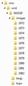
Individual image outputs
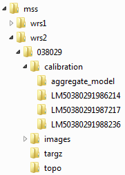
During the preparation of MSS, TM/ETM+, and OLI images for a given scene, a new directory called images is created with subdirectories for each year of imagery (Figure 6). Additionally for MSS scenes, a topo folder is created that contains the resampled and reprojected DEM file and derived slope and aspect files with properties that correspond to the MSS data.
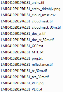
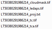
Within the individual year folders, a series of image and ancillary files are produced for each date in that year. Filenames contain the Landsat image ID code and a unique descriptor. Each MSS image has 15 associated files (Figure 7), TM/ETM+ images have 5 (Figure 8), as do OLI images (Figure 9). Table 2 (MSS), Table 3 (TM/ETM+), and Table 4 (OLI) describe what each file is and what LLR function (see Figure 2) creates it.
| File | Description | Function |
|---|---|---|
| archv.tif | 4-band MSS DN image | MSSunpackr (LPGS L1T MSS image) |
| archv_drkobjv.png | Histogram-based dark object selection assessment aid | MSScost |
| cloud_rmse.csv | Percent cloud cover and georegistration RMSE information | MSSunpackr |
| cloudmask.tif | 1-band cloud/shadow mask image. 0=clouds/shadow, 1=clear-view | MSScvm |
| cloudmask_30m.tif | 1-band cloud/shadow mask image resampled to 30m | MSScal |
| dos_sr.tif | 4-band MSS surface reflectance image | MSScost |
| dos_sr_30m.tif | 4-band MSS surface reflectance image resampled to 30m | MSScal |
| GCP.txt | Ground control points used in USGS LPGS processing | MSSunpackr (from LPGS processing) |
| MTL.txt | Image metadata | MSSunpackr (from LPGS processing) |
| proj.txt | PROJ.4 image projection definition | MSSunpackr |
| reflectance.tif | 4-band MSS TOA reflectance image | MSSdn2refl |
| tc_30m.tif | 3-band MSS tasseled cap image (brightness, greenness, wetness) | MSScal |
| tca_30m.tif | 1-band MSS tasseled cap angle image | MSScal |
| VER.jpg | Verify Image Product from USGS LPGS processing (georegistration information) | MSSunpackr (from LPGS processing) |
| VER.txt | Verify Image Product from USGS LPGS processing (georegistration information) | MSSunpackr (from LPGS processing) |
| File | Description | Function |
|---|---|---|
| cloudmask.tif | 1-band cloud/shadow mask image. 0=clouds/shadow, 1=clear-view | TMunpackr (FMask) |
| ledaps.tif | 6-band TM/ETM+ surface reflectance image from LEDAPS | TMunpackr (LEDAPS image) |
| proj.txt | PROJ.4 image projection definition | TMunpackr |
| tc.tif | 3-band TM/ETM+ tasseled cap image (brightness, greenness, wetness) | TMunpackr |
| tca.tif | 1-band TM/ETM+ tasseled cap angle image | TMunpackr |
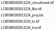
| File | Description | Function |
|---|---|---|
| cloudmask.tif | 1-band cloud/shadow mask image. 0=clouds/shadow, 1=clear-view | OLIunpackr (FMask) |
| l8sr.tif | 6-band OLI surface reflectance image from L8SR | OLIunpackr (L8SR image) |
| proj.txt | PROJ.4 image projection definition | OLIunpackr |
| tc.tif | 3-band OLI tasseled cap image (brightness, greenness, wetness) | OLIcal |
| tca.tif | 1-band TM/ETM+ tasseled cap angle image | OLIcal |
Calibration outputs
MSS WRS-2 images spectrally tie all intersecting MSS images to the TM images for a given scene. Landsat satellites 4 and 5 carried both MSS and TM sensors and from 1982 to 1992 collected images coincidently. These coincident image pairs provide an excellent dataset to calibrate the MSS data to TM data. Currently, linear models for each coincident pair are developed, as well as an aggregated model that combines a sample of pixels from each pair together in one model. The single models are compared against the aggregated model for evaluation purposes, but in the end only the aggregated model is used to calibrate MSS images to TM images. The same process is applied to calibrate the OLI data to ETM+ data, however, the population of coincident images between OLI and ETM+ are limited to a small set of overflight test images. Instead, we use the nearest date between a given OLI and ETM+ image as calibration pairs.
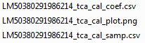
| File | Description | Function |
|---|---|---|
| *cal_coef.csv | Linear model coefficients for deriving TM index from MSS bands | MSScal/OLIcal |
| *cal_plot.png | Scatterplot showing relationship between MSS-modeled index and TM index | MSScal/OLIcal |
| *cal_samp.csv | Table of sample values from MSS and TM used to develop linear model | MSScal/OLIcal |
Besides the individual image-pair model folders there is a composite_model folder that contains diagnostic files related to the aggregate models (Figure 12).
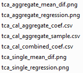
| File | Description | Function |
|---|---|---|
| *aggregate_mean_dif.png | Figure showing the difference between mean predicted index values (based on aggregate model) and actual values for each image used in model building | MSScal/OLIcal |
| *aggregate_regression.png | Scatterplot showing relationship between MSS/OLI-modeled index values and TM/ETM+ index values | MSScal/OLIcal |
| *cal_aggregate_coef.csv | Aggregated image-pair linear model coefficients for deriving TM/ETM+ TC index from MSS/OLI bands | MSScal/OLIcal |
| *cal_aggregate_sample.csv | Table of aggregated image-pair sample values from MSS/OLI and TM/ETM+ used to develop linear model | MSScal/OLIcal |
| *cal_combined_coef.csv | List of all individual image-pair linear model coefficients for deriving TM/ETM+ TC index from MSS/OLI bands | MSScal/OLIcal |
| *single_mean_dif.png | Figure showing the difference between mean predicted index values (based on single pair models) and actual values for each image used in model building | MSScal/OLIcal |
| *single_regression.png | Table of sample values from MSS and TM used to develop linear model | MSScal/OLIcal |
Composite outputs
The final step of LLR creates annual cloud free composites by applying image cloud masks (includes masking ETM+ bad scan lines) and merging multiple overlapping images from the same year into a single image using the mean. It produces a set of files for each TC index as individual year composite images and also as a temporal stack. The composite output directory is specified by the user (Running LLR Step 6 - Composite imagery) along with a unique composite identification string that is included in all file names for a given study area composite set. A subset example of the output files are shown Figure 13 and Table 7 describes what each file is. All file names adhere to the following naming convention:
Example: 2013_test_tca_composite.bsq
<year>_<unique ID>_<spectral index>_<descriptor>_<extension>
Where:
year = the year of the image composite
unique ID = the user-provided name of the composite series requested upon running the Step 4 of LLR
spectral index = the spectral index of the composite series
descriptor = a string describing the file
extension = file extension
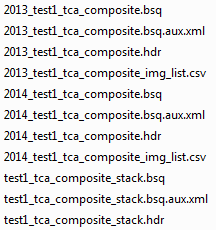
| File | Description | Function |
|---|---|---|
| <year>_<id>_<index>_composite.bsq | Image composite for a given year - ENVI file type | miXel |
| <year>_<id>_<index>_composite.bsq.aux.xml | Metadata for the corresponding composite image produced by default when writing ENVI files | miXel |
| <year>_<id>_<index>_composite.hdr | ENVI header file - needs to always accompany the corresponding .bsq image file | miXel |
| <year>_<id>_<index>_composite_img_list.csv | A list of individual images that went into creating the composite for a given year | miXel |
| <id>_<index>_composite.bsq | Annual image composite stack with as many bands as there are years. The bands are in acceding order of years ie low band number = early year and high band number = late year | miXel |
| <id>_<index>_composite.bsq.aux.xml | Metadata for the corresponding composite image produced by default when writing ENVI files | miXel |
| <id>_<index>_composite.hdr | ENVI header file - needs to always accompany the corresponding .bsq image file | miXel |
Helper functions
Mosaic DEMS
The mosaic_dems function will take an assemblage of adjacent DEM files and mosaic them together. MSScvm
cloud masking relies on a DEM to help identify water and remove topographic illumination variation.
This function is an easy way to create these DEM files. The function is called from the RStudio command prompt as:
mosaic_dems(dir, proj)
Where:
dir is the full path to a directory containing the individual DEM files that you wish to mosaic. The only files in the directory should be decompressed DEM files (no zipped files). proj is the PROJ.4 string that defines the common projection for all image data in your project. See the Selecting a geographic projection section for more information.
Example:
mosaic_dems(dir = "E:/dems/wrs1/045030", proj = "+proj=aea +lat_1=29.5 +lat_2=45.5 +lat_0=23 +lon_0=-96 +x_0=0 +y_0=0 +ellps=GRS80 +datum=NAD83 +units=m +no_defs")